Learning from LiDAR Data with Deep Learning

Lidar has been making headlines, from discovering lost Mayan ruins to aiding self-driving car navigation. Lidar is even in your new iPhone. But what exactly is lidar, and how can we leverage it in our existing deep learning toolbox?

A lidar sensor uses a laser pulse to create a 3D representation of a scene. The laser pulse hits an object, reflects back, and then the sensor measures the amplitude and time of the returned pulse. If we know the time of transmission, time of return, and speed of light, it is trivial to calculate the distance from the sensor to the object. We can leverage this by moving the laser in a scanning direction and collecting millions of these points to display an entire 3D scene, where each point represents the presence of an object at that location. This collection of points is called a point cloud.

A point cloud is one of the simplest data types there is. It is just a list of points containing X, Y, and Z values. However, point clouds have some qualities that distinguish them from images.

1. Permutation Invariance: The set of points is unordered. We can randomly vary the indices, and the point cloud will still represent the same scene. 
   
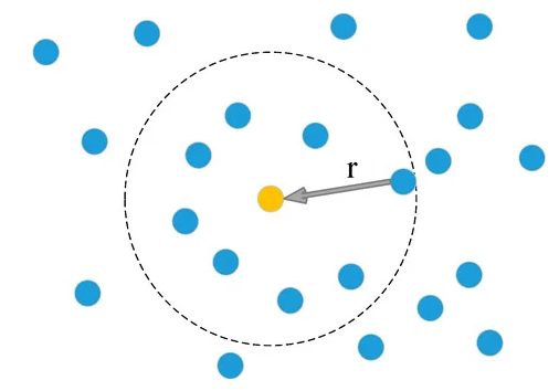
2. Distanced-based Neighborhood: Each point in a point cloud exists independently. In an image, the neighbors of a pixel can be determined by indexing, but in a point cloud, neighborhoods must be determined by distance.



3. Resolution Inconsistency: Resolution (or the number of points in a given volume) can vary widely throughout a scene. Typically objects close to the sensor have a dense resolution, while objects further away are sparse.

Although the 3D point cloud differs from a 2D image, the processing tasks, like object detection, semantic segmentation, and classification, remain the same. Historically, CNN's have had tremendous success as feature extractors in vision tasks for 2D images. However, the fundamental differences in the datatypes mean that we must make several critical changes to established CNN architectures to make them work for point clouds. This article will focus specifically on changes to the convolution operation.

2D Convolutions and their Role in CNNs

Convolution is an operation between two functions. In the image processing space, the two functions are the image itself and a kernel. The convolution operation takes place as follows:

For each pixel in the image

1. Place the kernel over the pixel
2. Multiple each value in the kernel by the pixel it is overlapping
3. Sum up the multiplied values and assign this new value to the center pixel location.

While the convolution operation is quite simple, it is excellent for extracting local features and is equivariant to translation (an essential quality for image processing). In addition, convolution also has a few computational attributes that make it desirable for image processing.

1. Sparse connectivity: Traditionally, the kernel is several sizes of magnitude larger than the image and requires only the information from a few neighboring pixels. This sparse connectivity allows for fast operations and parallelization.
2. Small Number of Parameters: The kernel is a function whose values are used repeatedly at each pixel location. This repeated use significantly reduces the number of parameters needed and the storage requirements of the model. The parameters will also be consistent, no matter the input size.

Convolutions are great, and they are an obvious choice for feature extraction. However, a few critical differences between images and point clouds make it impossible to use traditional convolution directly on point clouds. Let's examine some of those differences.

1. Convolutions rely on the order of the data. An image is dependent on a specific order of the pixels. A point cloud however, has no order dependencies.
2. Convolution requires well-defined neighbors that we can easily access via indexing. Images rely on the receptive field of the kernel, which we can infer. Point clouds depend on the distance, which we must calculate directly.
3. Convolution relies on a consistent resolution. Images are dense and have consistent and uniform data. Point clouds, however, are sparse and have inconsistent and unorganized data.

Any variations of the convolutional operation must be invariant to the order of the points AND take the points' spatial location and resolution into account. This paper provides an excellent overview of the enormous variety of convolution/feature extraction methods developed for point clouds. This work will focus on two of the most common point cloud-based strategies; Pointwise MLP(Multi-layer Perceptrons) and Point Cloud Convolution.

Pointwise MLP

Initial attempts to use convolutions with point clouds relied on transforming the point clouds into a secondary data type, like voxels or images. However, the Pointwise MLP recognizes the information loss of transforming into another data type and aims to operate on the point directly. This section will focus on the most popular Pointwise MLP solution, PointNet/PointNet++.

Pointnet first identifies a need for a symmetric function. A symmetric function is a function that produces the same output regardless of the order of the inputs. Examples of symmetric functions include mean, max and min. The symmetric function is vital because it maintains the property of permutation invariance. An infinite number of symmetric operations can be applied to a set of points and the result will be the same, regardless of point order.

PointNet aims to make a family of symmetric functions from neural networks; it consists of a shared MLP, a max pooling operation, and another MLP. This basic set of functions allows us to take a group of points and calculate a feature. Therefore, we can consider the output of PointNet a global feature for the entire point cloud.

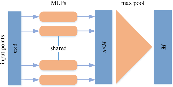
We need a combination of local and global features for many vision tasks. So we expand upon PointNet by introducing PointNet++. This simple extension proposes that we can calculate local features by calculating global features on small subsets or neighborhoods of these points. The steps are as follows:

1. Determine the desired dimension of the output point cloud. For various applications, upsampling, downsampling, or keeping the exact dimensions might be appropriate.
2. Group points together. For each point, get its neighbors by using a distance radius function or choosing a set number of nearest neighbors to your point of interest.
3. Calculate the features for each output point based on these local neighborhoods.

This method is one of the most common feature extraction techniques because it is a robust method that operates directly on the points themselves.

Pointwise Cloud Convolutions

While PointNet feature extraction is a widespread technique it has some downfalls, the first downfall is that within a point group, all points are weighted equally; there is no consideration or weighting for points that may be closer or farther away. The shared MLP can also lead to a large number of parameters. Because of these issues, we may want to consider another group of convolution operations called Point Cloud Convolutions. These operations have more direct similarities to traditional convolutions and can be much more efficient. This paper gives a great in-depth overview, but the basics are as follows.

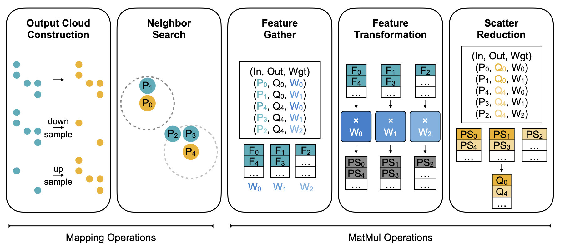
Point cloud convolutions have five primary steps:

1. Establishing the output point clouds

In this step, we perform operations that establish the output dimensions of the point clouds. For example, changes in dimension might include upsampling, downsampling, or keeping the same dimension.

2. Neighbor Search

We then find the local neighborhood of each point. Ball query search, kernel mapping, or nearest neighbor search are all popular choices.

3. Feature Gathering

Next, for each point of interest, we gather the feature maps associated with their neighboring point. These are all concatenated.

4. Feature transformation

The feature maps are then multiplied by the associated weights. At this step, consider adding weighting for point distance or sparsity.

5. Scatter Reduction

Finally, each result is associated with its final output, and partial sums are combined using a pooling or summation operation.

All point cloud convolution operations follow the same basic steps; however, there is plenty of room to tailor these to your particular dataset.

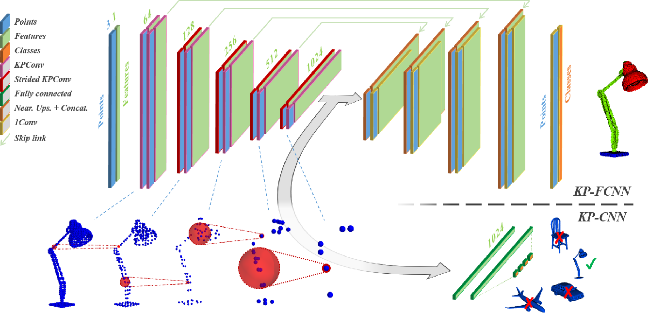
Once we have the point cloud convolution operation, the architecture remains essentially the same. Therefore, we can compare two semantic segmentation networks: UNet and KPConv. While the first is an image network and the second is a point cloud network, they follow the same overall strategy:

1. Downsampling layers, each downsampling spatial size while increasing feature dimensions
2. Upsampling layers, increasing spatial size while decreasing feature dimensions
3. Shared information between upsampling and downsampling layers of the same size
4. Output segmentation map of the same size as the input

The only significant changes are the convolution operations!

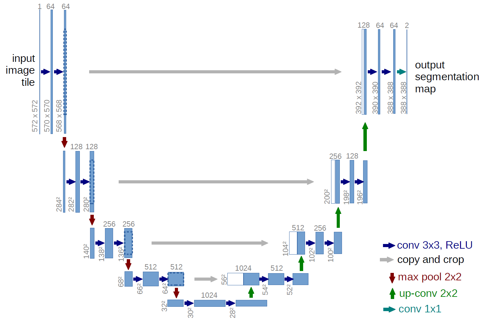
Although there are significant differences between 2D images and 3D point clouds, the architectures and applications are primarily the same. Therefore, once we know the peculiarities of the point cloud data type, we can start building a toolbox of equivalent functions and substitute them into our existing architectures as necessary, just like we have demonstrated here with the convolution function.